What We’re Working On
A Visual Image that Might be Created by Spiking Neuromorphic Neurons
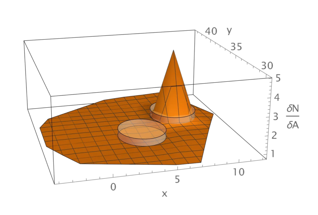
A random sample of 500 coordinate values of a line drawing were used to determine visual positions of 500 neurons that produced phosphenes. An additional 500 neurons provided a dark background. Spikes were generated using code that provided pseudorandom spike times for a constant frequency of 90 spikes/s. It was assumed that the occurrence of a spike activated synapses for which each neuron was presynaptic, and that synapses remained in an active state for 10 ms. An update interval of 0.05 ms was used to detect times at which the synapses made by each neuron were active. Images of phosphenes created for each update included only those neurons for which the synapses were active.
Articles
Training a Feedforward Neural Network (FFNN) to Make Explicit Information Regarding Phosphene Distributions in Spike Frequency Distributions


The darker circles in the graphic on the right depict the 49 visual columns that were simulated, and the columns containing red disks received simulated stimulation on selected simulations. Column 12 is the leftmost column containing a red disk. From bottom to top, the remaining columns with red disks are 4, 1, and 5.
The graphic on the left shows the corresponding visual regions, assuming that the simulation was based on what we refer to as the normal visual geometry. Region 12 appears in the lowest position. From left to right, the remaining regions containing red disks are 5, 1, and 4.

What follows is a description of the central idea underlying the feedforward network (FFN). Neurons in each column of the V1 network send output to neurons in every column of the FFN Layer 1. This all-to-all projection also holds from the output of FFN Layer 1 to FFN Layer 2.
In the normal visual geometry, each visual region corresponds to exactly one column. If a phosphene is expected on region Ri, then we want the neuron in Ci of FFN Layer 2 to produce spikes at the maximum rate, and all other neurons not to produce any spikes.
In the unified visual geometry, regions R4 and R5 are each set equal to the union of normal geometry regions R1 and R4 and R5. If C1 is stimulated, then a phosphene is expected only on R1, and we want only the neuron in C1 of FFN Layer 2 to produce spikes at the maximum rate. However, if C4 or C5 is stimulated, then a phosphene is expected on normal geometry regions R1 and R4 and R5. In this case, we want the neurons in C1 and C4 and C5 of FFN Layer 2 to produce spikes at the maximum rate.
The 49 simulated columns of visual cortex each contain 4 excitatory neurons and 2 inhibitory neurons. In order to train the FFNN, a 98-element vector of numbers of spikes in each 1s interval is created for each of the 8 possible pairs of 1 excitatory and 1 inhibitory neuron. There are 10, 1s intervals in a simulation and 13 stimulation conditions, yielding 80 x 13 = 1040 possible input vectors for each normal or unified visual geometry training session. We will report FFNN performance for simulation data from combined normal and unified visual geometry conditions. For this case, the FFNN was trained with 2080 input vectors. In each case, the number of spikes is scaled to lie in the interval [-10,10].
Neurons in each of two layers are comprised of a set of trainable weights followed by a logistic sigmoid function. The first layer consists of 98 neurons, each receiving synaptic inputs from all 98 elements of the input vector. Each neuron in this layer implements the dot product w • x, where x is the input vector and w is a weight vector originally set to random values in the interval [0,1]. The dot product of the two vectors forms the input to a logistic sigmoid function with an output codomain in the interval [0,1].
The 98-element vector output of the first layer forms the input to a second layer in which each of 49 neurons is again composed of a linear weighting function followed by a logistic sigmoid function. Each of these neurons receives weighted input from all 98 elements of the first layer output, and produces an output in the interval [0,1].
Each 98-element input vector is paired with a 49-element training vector. An element of the training vector for each simulation condition is set to 1 if its index corresponds to a visual region on which a phosphene is expected to appear, and to 0 otherwise.
The following table displays index values of cortical columns corresponding to visual regions on which phosphenes are expected to appear. The same index values also refer to output layer neurons that are trained to produce an output value of 1.

“NET” is used to describe simulations of the neural network that do not include the neuromorphic device. “NEURO” is used for simulations that include the device. Each simulation was run using 40, 50, or 60 excitatory spikes/s delivered to all excitatory network neurons.
Columns 1, 4, 5, and 12 are labeled C1, C4, C5, and C12. “All Others” refers to indices of the remaining 45 columns. x-bar denotes the mean scaled spike frequency for C1, C4, C5, and C12. It denotes the overall mean scaled spike frequency over the remaining 45 columns. m and M denote the minimum and maximum frequency values for neurons that correspond to c1, c4, c5, and c12. They denote the average minimum and maximum frequency values for neurons that correspond to the remaining 45 columns.
Output values were multiplied by 100 so that they lie in a spike frequency interval [0,100]. All values are shown to 5 digit precision.


PAPER IN PREPARATION
We have extended our simulations of neurons in 49 cortical columns to include a neuromorphic device that intermittently records from and stimulates 4 cortical columns. The device is meant to create a second, desired visual geometry in which discrete phosphenes are unified. Multinomial logistic regression analyses of spike frequency distributions from simulations that do and do not include the device classify expected numbers of phosphenes with accuracy greater than 99%. This result is important because it demonstrates that adding a second, desired visual geometry with the goal of unifying discrete phosphenes alters spike frequency distributions in a way that permits correct classification of the number of expected phosphenes.
We have performed additional multinomial logistic regression analyses of spike frequency distributions which classify expected perceptions of local lightness maxima (phosphenes) on one or more regions of the visual geometry (locations in visual space). The lowest classification accuracy is 98.99% correct for a control parameter value of 40 spikes/s. Accuracy is 100% correct for control parameter values of 50 spikes/s and 60 spikes/s. These results are important because it seems likely that information on local lightness maxima on regions of the visual geometry underlies classifications of the number of phosphenes.
We have devised three methods of visualizing spike frequency distributions in an effort to understand properties of the distributions that underlie the above classifications. One method demonstrates that distributions contain information on the column or columns which receive electrical stimulation above the phosphene threshold. This information is exceptionally clear when the control parameter = 60 spikes/s, as shown by the example labeled Figure A. The second method reveals differences between distributions that are produced by changes in synaptic strengths that are introduced in order to alter the visual geometry and thereby unify discrete phosphenes. This method is illustrated by the example labeled Figure B. The third method reveals the dominant difference or differences between distributions that are produced by altering synaptic strengths. This method is illustrated by the example labeled Figure C. All three methods are effective for network alone simulations and for simulations that include the neuromorphic device. These results are important because knowing the columns stimulated and the visual geometry is sufficient for identification of local lightness maxima on regions of the visual geometry.
Please see https://doi.org/10.3390/prosthesis4040049 and https://zenodo.org/record/8102357 for details of the models and simulations used to produce these results.
Normal Geometry
Altered Geometry
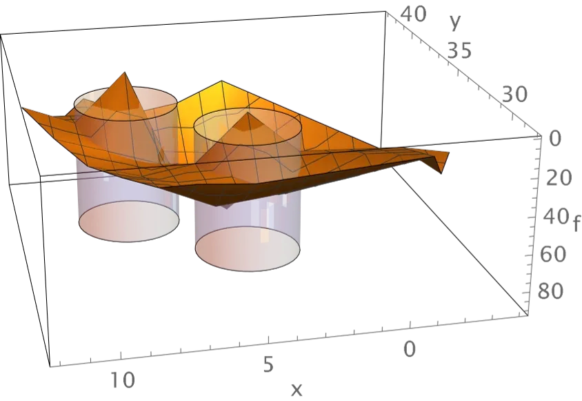
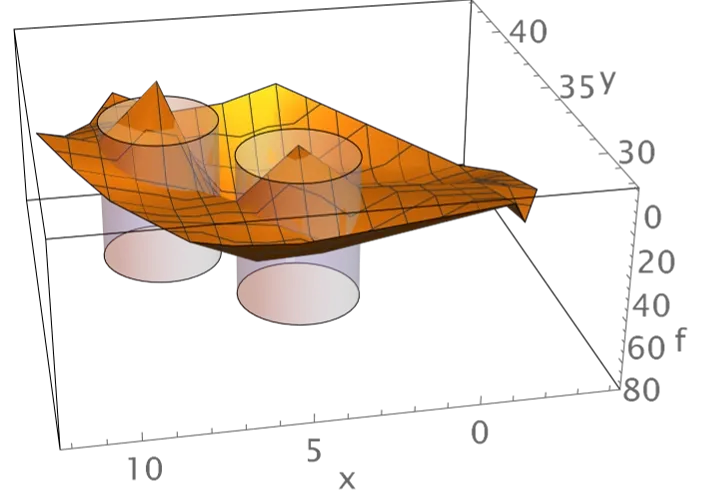
Figure A
Surfaces estimated from mean excitatory neuron spike frequencies for simulations of 10 seconds duration are shown for the case of stimulation of columns 5 and 12. The data are from simulations that include the neuromorphic device. The locations of columns 5 and 12 are highlighted using semi-transparent cylinders. Note that the graphic has been rotated through 180° (turned upside down) in order to reveal the low frequencies in stimulated columns. This visualization is made possible by subtracting mean spike frequencies obtained from simulations in which no columns receive above phosphene threshold stimulation. The graphic in the top panel illustrates frequencies for simulations that use the normal geometry, and the graphic in the bottom panel illustrates frequencies for simulations that use an altered geometry in which synaptic strengths have been changed so that the visual regions corresponding to columns 4 and 5 are each set equal to the union of regions 1 and 4 and 5.
Figure B
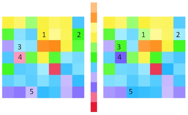

Array plots are shown for the mean excitatory frequencies depicted in Figure A in order to make possible visualization of differences between the frequency distributions for the normal (left) and altered (right) visual geometry data. The correspondence between column numbers and positions in the arrays are given in the table in the rightmost panel of this figure. The color spectrum shown between the colored array graphics is anchored to the minimum and maximum frequencies for all stimulation conditions. Note that neurons in columns 5 and 12 have the lowest frequencies. The positions in the arrays that are labeled using the integers 1-5 are examples of visually obvious differences in frequencies that arise from differences in the visual geometries.